How to Get Fit and Learn Data Science at the Same Time
A Short Introductory Data Project Using R
November 1st, 2020
While majoring in Economics during undergrad, I heard the term 'Data Science' thrown around constantly. It seemed like THE skill to have when looking for jobs/ internships. I wanted to learn how to code but was intimidated, not knowing where to start. If you’re like me, self-directed study is difficult when you have so much else on your plate. I checked out a handful of the online resources that were recommended to me by friends, but nothing really got me motivated to learn. What I needed was a project; a task to sink my teeth into and produce results.
Aside from learning to code, something I never found time for in college was working out. I was one of those people who started out every term with a fitness goal that was promptly abandoned after midterms. It occurred to me that I could combine these areas that I was lacking in and kill two birds with one stone. I simply decided to keep track of the time I spent exercising and create some visualizations of that data. As it turned out, this strategy was quite effective at getting me motivated to work towards both my fitness and data science goals. Here are the steps that I took:
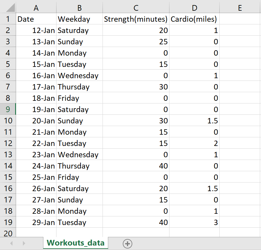
1) Start working out! Keep track of your progress on an excel sheet formatted like this:
Save your table as a CSV (Comma delimited) file into a folder you should create that is dedicated to this project.
2) On the days you’re not getting swole, consider reading
R for Data Science:
This book serves as a great introduction to R. In the first few chapters it teaches you how to download R and make simple visualizations.
a. For instructions on downloading R go to R for data science > Introduction > Prerequisites. You'll need to download both R and RStudio.
b. Reading sections 1.4 – 1.5 and 3.1 – 3.3 should be enough to get you prepared for this project.
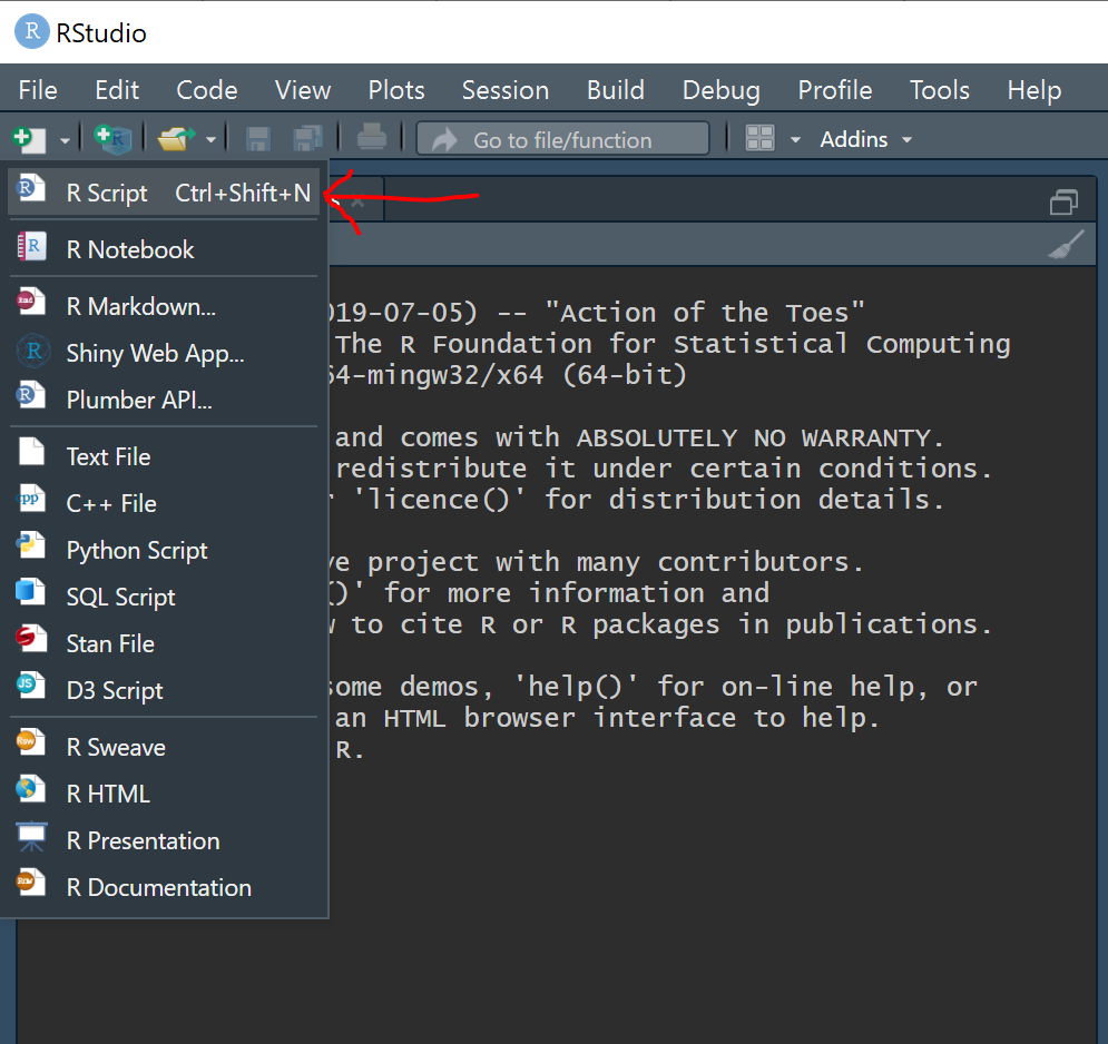
3) Open RStudio and create a new
R script by navigating to the drop down menu at the top left (the white square with the plus sign).
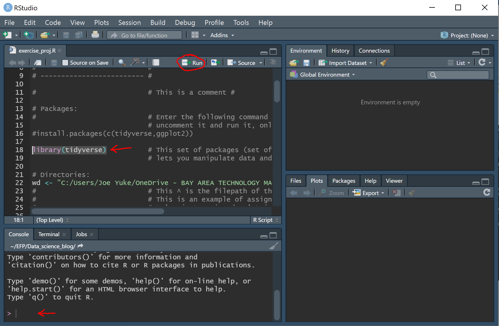
a. Note that there are 2 different ways to run code in R:
i. Enter lines of code directly into the Console at the bottom left.
ii. Highlight lines of code from your script and hit the ‘Run’ button.
Lines of code written in the script can be saved for later whereas lines written in the console cannot. Practice running 1 + 1 each way.
c. Note that it’s always good practice to mark up your programs with Comments. Any line or part of a line that has # in front of it is commented out which means it is only meant to be read by the user. R is not able to run commented lines of code.
4) Install and load packages:
A
Package contains functions for use in your program. The package that we will focus on,
tidyverse, is actually a group of different packages that allow us to clean data and create plots. To use the package, you’ll need to run the following lines of code:
install.packages("tidyverse")
library(tidyverse)
You only need to install a package one time; however, you will need to load in the package using the library() command in each new session of R.
(You might have to wait a while for tidyverse to install, don't fret)
5) Change working directory:
a. Locate the folder you’ve created for this project and copy the file path. It should look something like this for PCs:
C:/Users/Joe Yuke/Documents/EFP/workout_project
For Mac:
~/Users/Joe Yuke/Documents/EFP/workout_project
(Make sure to use foreward slashes in R when refering to file paths)
b. A fundamental statement in all coding languages is the Assignment statement which assigns a specified value to a variable you create. We’ll now assign the file path to the variable 'wd'.
wd <- "C:/Users/Joe Yuke/Documents/EFP/workout_project"
Once you’ve assigned the variable, it will appear in the Environment at the top right. You can now use it in other functions.
For example, try typing out the command: print(wd)
c. Next, set your Working Directory with the following function:
setwd(wd)
This tells R where you’re working out of for this project i.e. where you’re pulling data from and where to output your plots once you’ve made them.
6) Load in data:
a. For this step, we’ll use the function: read.csv() . So first, let’s look at the Help file for this function to see how to use it.
?read.csv
We're interested in seeing which Parameters (statements within the parentheses of the function) are required. Here's what we get:
read.csv(file, header = TRUE, sep = ",", quote = "\"", dec = ".", fill = TRUE, comment.char = "", ...)
This tells us that when calling the function, we only need to specify which file we’re pulling our data from. With the way our data is structured, we want to have a header, but the ‘header’ parameter is set to TRUE by default so we can leave it. The rest of the defaults are fine, so we’ll leave those too.
b. Run the following code to turn our .csv file into a Data Frame in R:
workout_data <- read.csv("Workouts_data.csv”)
c. It's helpful to check the data in R to see if it downloaded correctly. Click on 'workout_data' in the environment and see if it matches what we have on excel.
7) (Optional) Analyze data:
a. A simple analysis we might want to conduct is to see how many observations we have in our data. The following code helps us do this:
length(workout_data$Date)
The 'length' function returns the number of objects in a vector. The vector we want to look at is the list of dates in our data frame. To extract just the date variable, we make use of the '$' operator which allows us to extract elements by name from a named list.
Thus, this line tells us how many dates we have in our data frame.
b. It is also useful to know the Data Type of the objects in our data. Some functions only accept certain types of data. To check our data, we’ll isolate specific entries by using the Subset operator: ‘[ ]’. The first number in the brackets refers to the row we are interested in, the second refers to the column.
typeof(workout_data[1,3])
Running this line should tell us that the type of the object in the 1st row and 3rd column is an integer. This is fine since this object refers to the number of minutes spent working out on the first day. (Run: workout_data[1,3] , to see exactly how many minutes this is).
typeof(workout_data[,1])
Running this line tells us that the type of all the entries in the 1st column of our data are integers. However, we don’t want dates stored as integers. This will be a problem when creating our plots, so we will have to change the 'Date' variable into the date data type.
(Extra: try running this and see what happens: workout_data$Date[1:3] )
8) Edit data:
a. To format our dates correctly, change the 'Date' variable into the Date data type:
workout_data$Date <- paste("2019", workout_data$Date, sep="-")
workout_data$Date <- as.Date(workout_data$Date, format="%Y-%d-%b")
Briefly, the 'paste' function serves to add the string "2019" onto the beginning of each entry in the vector of dates and is separated by "-" each time via the 'sep' parameter. Next, 'as.Date' changes each date into the desirable data type. We specify using the 'format' parameter how we'd like the date to appear. Check out this guide for more information:
https://www.statmethods.net/input/dates.html
b. Suppose we realize that we overstated how much we ran on some day. To correct this mistake, we can edit a single observation by assigning a new value to the desired cell.
workout_data[18,4] <- 2.0
This type of command should be familiar by now. Take a look at the data frame to see if your change was made successfully.
c. Let’s also change the names of some of the variables in our data frame:
colnames(workout_data)[3:4] <- c("Strength Minutes","Miles Ran")
This line transforms the names of the 3rd to 4th columns through assignment of a vector of 2 string objects.
colnames() identifies the names of the variables, and c() creates a Vector of multiple objects separated by ','.
d. Add a new row by first creating a list. Lists are basically vectors that can include objects of different types. We need the entries in our new row to be of the same type as their respective column.
new_row <- list("2019-01-30", "Wednesday", as.integer(20), as.numeric(1.0))
workout_data <- rbind(workout_data,new_row)
The rbind() function then adds 'new_row' to the bottom of 'workout_data'.
9) Try out different types of graphs:
a. ggplot() is the function for creating plots. When you use it, you must specify a Geom- the type of graph. For our project, we'll make some bar graphs with geom_col(). Try running the following lines one at a time and see what happens:
(Two lines of code separated by '+' should be thought of as one line)
ggplot() +
geom_col(data=workout_data, aes(x=Date, y=`Strength Minutes`), fill="dodgerblue")
ggplot() +
geom_col(data=workout_data, aes(x=Date, y=`Miles Ran`), fill="salmon")
As you can see, we are specifying the data we're using, which variables we want on the x-axis and y-axis, and the color (fill) we want our bars to be.
(Note that ` is not the same as ', and is used when referring to a variable with spaces in its name like `Strength Minutes`)
b. We also need to specify the Aesthetics we want to use.
From the help file for aes(): Aesthetic mappings describe how variables in the data are mapped to visual properties (aesthetics) of geoms.
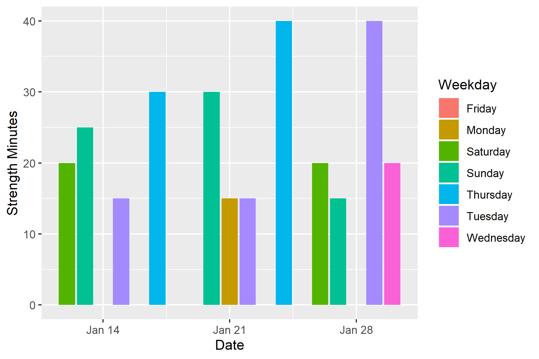
To illustrate its purpose, let's change the bar color to represent day of the week by including 'fill=Weekday' in aes():
ggplot() +
geom_col(data=workout_data, aes(x=Date, y=`Strength Minutes`, fill=Weekday))
We should get something that looks like this:
c. Lastly, we use ggsave() to create image files for our plots:
First, we assign a name to our plot, 'my_plot', then use the ggsave() function.
my_plot <- ggplot() +
geom_col(data=workout_data, aes(x=Date, y=`Strength Minutes`, fill=Weekday))
ggsave(paste(wd,"strength_plot.png", sep="/"), my_plot, height=4, width=6)
ggsave() requires us to input the full path of the image file we want to create, so we use the paste() function again.
10) Become a couch potato again:
Congratulations on completing your first project! Hopefully you've learned something from this experience. Obviously, data science goes waaaaay beyond the scope of this blog, but it should be a good place to start.
If you want to keep working, I recommend you read more of
R for Data Science and try out some of the new things you learn with this data, or find some new data to work with. Also, if you ever run into a coding problem you can't get past, you can look up pretty much any question about R on Google and the odds are that someone has already asked the same question.
Here are more resources to check out:
